DSA Time Complexity for Specific Algorithms
See this page for a general explanation of what time complexity is.
Quicksort Time Complexity
The Quicksort algorithm chooses a value as the 'pivot' element, and moves the other values so that higher values are on the right of the pivot element, and lower values are on the left of the pivot element.
The Quicksort algorithm then continues to sort the sub-arrays on the left and right side of the pivot element recursively until the array is sorted.
Worst Case
To find the time complexity for Quicksort, we can start by looking at the worst case scenario.
The worst case scenario for Quicksort is if the array is already sorted. In such a scenario, there is only one sub-array after each recursive call, and new sub-arrays are only one element shorter than the previous array.
This means that Quicksort must call itself recursively \(n\) times, and each time it must do \(\frac{n}{2}\) comparisons on average.
Worst case time complexity is:
\[ O(n \cdot \frac{n}{2}) = \underline{\underline{O(n^2)}} \]
Average Case
On average, Quicksort is actually much faster.
Quicksort is fast on average because the array is split approximately in half each time Quicksort runs recursively, and so the size of the sub-arrays decrease really fast, which means that not so many recursive calls are needed, and Quicksort can finish sooner than in the worst case scenario.
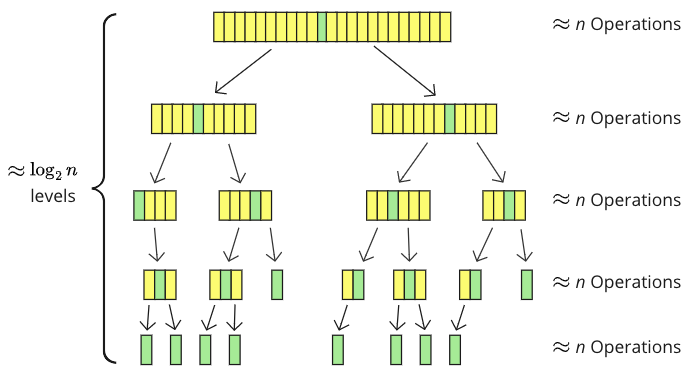
The image below shows how an array of 23 values is split into sub-arrays when sorted with Quicksort.

The pivot element (green) is moved into the middle, and the array is split into sub-arrays (yellow). There are 5 recursion levels with smaller and smaller sub-arrays, where about \(n\) values are touched somehow on each level: compared, or moved, or both.
\( \log_2 \) tells us how many times a number can be split in 2, so \( \log_2 \) is a good estimate for how many levels of recursions there are. \( \log_2(23) \approx 4.5 \) which is a good enough approximation of the number of recursion levels in the specific example above.
In reality, the sub-arrays are not split exactly in half each time, and there are not exactly \(n\) values compared or moved on each level, but we can say that this is the average case to find the time complexity:
\[ \underline{\underline{O(n \cdot \log_2n)}} \]
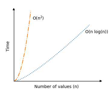
Below you can see the significant improvement in time complexity for Quicksort in an average scenario, compared to the previous sorting algorithms Bubble, Selection and Insertion Sort:

The recursion part of the Quicksort algorithm is actually a reason why the average sorting scenario is so fast, because for good picks of the pivot element, the array will be split in half somewhat evenly each time the algorithm calls itself. So the number of recursive calls do not double, even if the number of values \(n \) double.
Quicksort Simulation
Use the simulation below to see how the theoretical time complexity \(O(n^2)\) (red line) compares with the number of operations of actual Quicksort runs.
{{ this.userX }}
Operations: {{ operations }}
The red line above represents the theoretical upper bound time complexity \(O(n^2)\) for the worst case scenario, and the green line represents the average case scenario time complexity with random values \(O(n \log_2n)\).
For Quicksort, there is a big difference between average random case scenarios and scenarios where arrays are already sorted. You can see that by running the different simulations above.
The reason why the already ascending sorted array needs so many operations is that it requires the most swapping of elements, because of the way it is implemented. In this case, the last element is chosen as the pivot element, and the last element is also the highest number. So all other values in every sub-array is swapped around to land on the left side of the pivot element (where they are positioned already).

